A real number is defined as one that has no i in it. An imaginary number is a real number times i (such as 4i). A complex number has both real and imaginary parts. Any complex number z can be written in the form x+iy where x and y are real numbers. x is the "real part" and y is the "imaginary part." For instance, 2+3i is a complex number.
The complex conjugate of a complex number, represented by a star next to the number, is the same real part but the negative imaginary part. So if z=2+3i then z*=2–3i. Note that the reverse is also true: if z=2–3i then z*=2+3i. So you always have two numbers that are complex conjugates of each other.
Real numbers can be graphed on a line (the number line). Complex numbers, since they have two separate components, are graphed on a plane called the "complex plane" where the real part is mapped to the x-axis, the imaginary part the y-axis. Every complex number exists at exactly one point on the complex plane: a few examples are given below.
Every complex number has a magnitude which gives its distance from the origin (0) on the complex plane. So 1 and i both have magnitude 1. The magnitude is written with absolute value signs. So we can say that if z=2+3i then |z|2=22+32.
If you multiply any number by its own complex conjugate, you get the magnitude of the number squared (you should be able to convince yourself of this pretty easily). So we can write that, for any z, z*z=|z|2.
[close]
Suppose you roll a 4-sided die. What number do you expect to get? Answer: you have no idea. Any number is as likely as any other, presumably.
Expectation Values
OK, but on average what number will you get? For instance, if you rolled the die a million times, and averaged all the results (divided the sum by a million), what would the answer probably be? This is called the "expectation value." You can probably see, intuitively, that the answer in this case is 2½. Never mind that an individual die roll can never come out 2½: on the average, we will land right in the middle of the 1-to-4 range, and that will be 2½.
But you can't guess the answer quite so easily if the odds are uneven. For instance, suppose the die is weighted so that we have a 1/2 chance of rolling a 1, a 1/4 chance of rolling a 2, a 1/8 chance of rolling a 3, and a 1/8 chance of rolling a 4? Your intuition should tell you that our average roll will now be a heck of a lot lower than 2½, since the lower numbers are much more likely. But exactly what will it be?
Well, let's roll a million dice, add them, and then divide by a million. How many 1s will we get? About 1/2 million. How many 2s? About 1/4 million. And we will get about 1/8 million each of 3s and 4s. So the total, when we add, will be (1/2 million)*1+(1/4 million)*2+(1/8 million)*3+(1/8 million)*4. And after we add—this is the kicker—we will divide the total by a million, so all those "millions" go away, and leave us with (1/2)1+(1/4)2+(1/8)3+(1/8)4=1 7/8.
The moral of the story is: to get the expectation value, you do a sum of each possible result multiplied by the probability of that result. This tells you what result you will find on average.
[close]
Before explaining Fourier transforms, we will start by quickly reviewing a related topic you may be more familiar with, namely Fourier series. If you have any function f(x) that is periodic with period L you can write it as a sum of sine and cosine terms:
Fourier Transforms
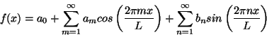
For each sine or cosine wave in this series the wavelength is given by L/m or L/n respectively. In other words the indices m and n indicate the wave number (one over wavelength) of each wave. Using the formula
eix=cos x + i sin x
you can rewrite the Fourier series in the equivalent form
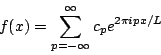
The function e2pipx/L is called a plane wave. Like a sine or cosine wave it has a value that oscillates periodically, only with plane waves this value is complex. That means that even if f(x) is a real function the coefficients cp will in general be complex. Either way you represent it, however, a Fourier series is simply a way of rewriting a periodic function f(x) as an infinite series of simple periodic functions with numerical coefficients.
A Fourier transform is the exact same thing, only f(x) doesn't have to be periodic. This means that the index p can now take on any real value instead of just integer values, and that the expansion is now an integral rather than a sum.
![]()
The factor of ![]() is a matter of convention and is set differently by different authors. Likewise some people add a factor (usually ±2p) in the exponential. The basic properties of the Fourier transform are unchanged by these differences. Note that this formula has nothing to do with position and momentum. The variable x could be position, or time, or anything else, and the variable p tells you the wave number (one over wavelength) of each plane wave in the expansion. (If x is time then the wave number is the same thing as the frequency of the wave.) To invert this formula, first multiply it by e—ip'x (where p' is just an arbitrary number) and then integrate with respect to x.
is a matter of convention and is set differently by different authors. Likewise some people add a factor (usually ±2p) in the exponential. The basic properties of the Fourier transform are unchanged by these differences. Note that this formula has nothing to do with position and momentum. The variable x could be position, or time, or anything else, and the variable p tells you the wave number (one over wavelength) of each plane wave in the expansion. (If x is time then the wave number is the same thing as the frequency of the wave.) To invert this formula, first multiply it by e—ip'x (where p' is just an arbitrary number) and then integrate with respect to x.
![]()
It is possible to evaluate the integrals on the right hand side of this equation, but doing so requires a familiarity with Dirac delta functions. If you are not familiar with these functions you can just skip the next paragraph and jump straight to the result. (We discuss Dirac delta functions in a later footnote, but if you're not already somewhat familiar with them trying to follow the argument below may be an exercise in frustration.)
The only x dependence in this integral comes in the exponential, which is an oscillatory function. If p-p' is anything other than zero then this exponential will have equal positive and negative contributions and the integral will come out to zero. (Actually eipx is complex so the equal contributions come from all directions in the complex plane. If you can't picture this just take our word for it.) If p-p' is zero, however, then the exponential is simply one everywhere and the x integral is infinite. Thus the x integral is a function of p-p' that is infinite at p-p', and zero everywhere else, which is to say a delta function. Of course this isn't a rigorous proof. It can be proven rigorously that the integral of a plane wave is a delta function, however, and when you do the math carefully you find that the integral produces a delta function with a coefficient of 2p. So
![]()
where the integration over p uses the defining characteristic of a delta function. Replacing the dummy variable name p' with p we finally arrive at the formula
![]()
We should emphasize once more that mathematically x is just the argument to the function f(x) and p is just the wave number of the plane waves in the expansion. The fact that the relationship between Y(x) and f(p) in quantum mechanics takes the form of a Fourier transform means that for a given wavefunction Y(x) the momentum happens to be inversely related to the wavelength. (Once again, though, a realistic wavefunction will be made of many waves with different wavelengths.)
We said before that the numerical coefficients in the Fourier transform definition were arbitrary. In quantum mechanics these coefficients pick up an extra factor of ![]() , so the full relation between Y(x) and f(p) is
, so the full relation between Y(x) and f(p) is
![]()
![]()
Finally, we should note one convenient theorem about Fourier transforms. Consider the normalization of the wavefunction, which is determined by the integral of its squared magnitude. Writing that in terms of the Fourier expansion we find
![]()
This result can be proven by taking the complex conjugate of the expression for Y(x) above, multiplying it by Y(x), and integrating over x using the same delta function trick we used above. We won't bother to show this proof here. Recall that f(p) is the coefficient of the momentum basis state with momentum p, so what this result says is that if the wavefunction is properly normalized so that the total probability of the position being anywhere is one, then it will automatically be normalized so that the total probability of the momentum having any value is one.
[close]
In classical physics a particle at any given moment has a position and a momentum. We may not know what they are, but they exist with some exact values. In quantum mechanics a particle has a wavefunction which gives it some probability distributions for position and momentum. The uncertainty principle says that the more definite position is the less definite the momentum, and vice-versa.
The Uncertainty Principle
We can see how this comes out of the rules we've given so far by considering the basis states of momentum, which are of the form eipx/![]() , which is equal to cos(px/
, which is equal to cos(px/![]() )+i sin(px/
)+i sin(px/![]() ). In other words the basis states of momentum are waves whose wavelength is determined by the value p. (Specifically, the wavelength is 2p
). In other words the basis states of momentum are waves whose wavelength is determined by the value p. (Specifically, the wavelength is 2p![]() /p.) When you expand a wavefunction in momentum basis states you are writing Y(x) as a superposition of these waves.
/p.) When you expand a wavefunction in momentum basis states you are writing Y(x) as a superposition of these waves.
Those familiar with Fourier expansions know that a localized wave is made up of components with many different wavelengths. At the other extreme a function made up of a single wave isn't localized at all. If a particle is in a momentum eigenstates Y=eipx/![]() then its position probabilities are equally spread out over all space. The bigger the range of wavelengths contained in the superposition the more localized the function Y(x) can be. From this we can see that a particle highly localized in momentum (a small range of wavelengths for Y) will have a very uncertain position (Y(x) spread out over a large area), and a particle highly localized in position (Y(x) concentrated near a point) will have a very uncertain momentum (many wavelengths contributing to the Fourier Transform of Y). You can certainly cook up a wavefunction with a large uncertainty in both position and momentum, or one that's highly localized in one but uncertain in the other, but you can't make one that's highly localized in both.
then its position probabilities are equally spread out over all space. The bigger the range of wavelengths contained in the superposition the more localized the function Y(x) can be. From this we can see that a particle highly localized in momentum (a small range of wavelengths for Y) will have a very uncertain position (Y(x) spread out over a large area), and a particle highly localized in position (Y(x) concentrated near a point) will have a very uncertain momentum (many wavelengths contributing to the Fourier Transform of Y). You can certainly cook up a wavefunction with a large uncertainty in both position and momentum, or one that's highly localized in one but uncertain in the other, but you can't make one that's highly localized in both.
It's possible to make a mathematical definition of what you mean by the uncertainty in position or momentum and use the properties of Fourier Transforms to make this rule more precise. The rule ends up being that the product of the position uncertainty times the momentum uncertainty must always be at least ![]() /2.
/2.
[close]
What does it mean to square an operator? It means "to do that operator twice." Why does it mean that? Really, it's just a matter of definition. So if D is the operator d/dx, then we say that D2f=d2f/dx2. It could just as easily have been defined some other way (for instance, as (df/dx)2) but it isn't: squaring an operator means doing it twice.
Squaring an Operator
OK, you say, but if it's that arbitrary, then why does it work? Why can we say that kinetic energy is p2/2m, so the kinetic energy operator will be found by squaring the momentum operator and then dividing by 2m? Well, to some extent, you have to accept the operators as postulates of the system. But it does make sense if you consider the special case of an operator corresponding to some observable acting on an eigenfunction. If Yp is an eigenfunction of momentum with eigenvalue p that means that a particle whose wavefunction is Yp must have a momentum of exactly p. In that case, though, its momentum squared must be exactly p2, which is the eigenvalue you get by acting on Yp with the momentum operator twice. So in the end, it's not quite as arbitrary as it first appears. (Of course, this is not a proof of anything, but hopefully it's a helpful hand-wave.)
[close]
To see why this works consider first the case where Y happens to be an eigenfunction of O with eigenvalue v. We know that a measurement of the quantity O will yield exactly v, so the expectation value of O must be v. We also know, however, that OY= vY, so the formula gives us
Where did the formula <O>=![]() Y*OYdx come from?
Y*OYdx come from?
![]()
where in the last step we've used the fact that the wavefunction must be normalized. For this special case we can see that our formula worked. What happens when Y is not an eigenfunction of O? For simplicity let's consider a wavefunction made up of just two basis states:
Y=C1Y1+C2Y2
We know for this case the correct answer for the expectation value of O is v1|C1|2+v2 |C2|2. To see how our formula gives us this result we act on Y with the operator O to get
OY=C1v1Y1+C2v2Y2
Our formula then tells us that
![]()
![]()
The first two terms look like exactly what we need since each basis state Yi is itself a valid wavefunction that must be properly normalized. (This is a bit more complicated for continuous variables, where the basis states are not normalized in this way, but a similar argument applies.) The last two terms seem to spoil the result, though. Here's the hand-waving part: for any two different basis states Y1 and Y2, the integral
![]()
will always be zero. The technical way to say this is that the basis states of all operators representing observables are orthogonal. This property, which we're not going to prove here, is the last necessary step to show why the expectation value formula works. (We do make an intuitive argument why this is true for the momentum basis states in our footnote on Fourier transforms.)
[close]
What is the basis function for position?
The Basis State of Position
The best way to answer this is actually not mathematically, but physically. Remember that a basis function represents a state where the particle has exactly one value, and no probability of being any other value. But we know that you find probabilities of position by squaring the wavefunction. So if we want a function that says "the position must be exactly 5" then clearly this wavefunction must equal 0 at every point but x=5. But if the probability distribution is completely concentrated at one point then it must be infinitely high at that point!
This function—infinitely high at one point, zero everywhere else—is known as the Dirac delta function and is written as the Greek letter delta. So d(x-5) is the function that is infinitely high at x=5, and zero everywhere else, such that the total integral is 1. To make this definition mathematically rigorous, you have to define it as a limiting case of a function that gets thinner-and-taller while keeping its integral at 1.
We said earlier that the position operator is x (meaning "multiply by x"). Now we're saying that the delta function is the position basis function: in other words, the eigenfunction for that operator. So it should be true, for instance, that xY=5Y when Y=d(5). In one sense we can see that this is true. Since d(x-5)=0 everywhere except x=5 multiplying it by x can only have an effect at the point x=5. So we can say that xd(x-5)=5d(x-5). At the same time, it seems kind of silly to multiply an infinitely large number by 5. What it really means is that the integral of the delta function, which was 1 by definition, will now be equal to 5.
Of course the above explanation isn't at all rigorous mathematically. In fact the "definition" we gave of the Dirac delta function was pretty hand-waving. The more rigorous definition involves taking the limit of a series of functions that get thinner and taller around x=5 while keeping their total integral equal to 1. If you think about multiplying one of these tall, narrow functions by x and then integrating you should be able to convince yourself that you get the same narrow function, only five times taller.
[close]
The simplest type of differential equation is an equation involving some function f(x) and its derivatives f'(x), f''(x), etc. Consider for example Newton's second law F=ma. In a typical situation you will know the force F acting on a particle as a function of that particle's position. Say the particle is a mass on a spring so that F=-kx. Then Newton's second law becomes the differential equation
Partial Differential Equations
x''(t)=-k/m x(t)
An equation like this is called an ordinary differential equation (ODE) because the dependent variable, namely the function x that you are solving for, depends only on one independent variable, t. You can write down a general solution to this equation, but it will necessarily have undetermined constants in it. Because this is a second order ODE it has two undetermined constants. The full solution of this particular equation is
x(t)=C1sin(![]() t)+C2cos(
t)+C2cos(![]() t)
t)
The undetermined constants C1 and C2 indicate that you can put any number there, and you will still have a solution: for instance, 2sin(![]() t)-¾cos(
t)-¾cos(![]() t) is one perfectly valid solution. To find the constants that should be used for a particular situation, you must specify two specific data, such as the initial conditions x(0) and x'(0). In other words if you know the state of your particle (position and velocity) at t=0 then you can solve for its state at any future time.
t) is one perfectly valid solution. To find the constants that should be used for a particular situation, you must specify two specific data, such as the initial conditions x(0) and x'(0). In other words if you know the state of your particle (position and velocity) at t=0 then you can solve for its state at any future time.
In quantum mechanics we have to deal with a partial differential equation (PDE), which is an equation where the dependent variable (Y in this case) depends on two independent variables (x and t). As a simple example of a PDE (simpler in some ways than Schrödinger's Equation) we can consider the wave equation
![]()
Here f(x,t) is some function of space and time (eg the height of a piece of string). Once again we can write down the general solution to this equation, but now instead of a couple of undetermined constants we have some entire undetermined functions!
f(x,t)=g1(x-t)+g2(x+t)
You can (and should) check for yourself that this solution works no matter what functions you put in for g1 and g2. You could write for example
f(x,t)=sin2(x-t)+ln(x+t)
and you would find that f satisfies the wave equation. How can you determine these functions? For the ODE above it was enough to specify two initial values, x(0) and x'(0). For this PDE we must specify two initial functions f(x,0) and f'(x,0) (where the prime here refers to a time derivative). For a piece of string, for instance, I must specify the height and velocity of each point on the string at time t=0, and then my solution to the wave equation can tell me the state of my system at any future time.
How does this apply to Schrödinger's Equation? Schrödinger's Equation is only first order in time derivatives, which means you can write the general solution in terms of only one undetermined function. In other words if I specify Y(x,0) that is enough to determine Y for all future times. (One way you can see this is by noting that if you know Y(x,0) Schrödinger's Equation tells you Y'(x,0), so it wouldn't be consistent to specify both of them separately.) So to solve for the evolution of a quantum system I must specify my initial wavefunction and then solve Schrödinger's Equation to see how it evolves in time.
[close]