You almost certainly don't want to read this entire page from start to finish. I do recommend you start by reading the entire "The Basics" section. But after that, use the "Contents" menu at the top to jump to specific topics you need.

And by the way...if you are a high school math teacher, the good folks at NumWorks will give you a free calculator just to encourage you to try their product. I got mine that way, which led to the writing of this page. They also have an online simulator (free for anyone to download): it's useful for demonstrating the calculator to your class, and it's also how I got all the awesome screen shots in this Web page.

---

The Basics

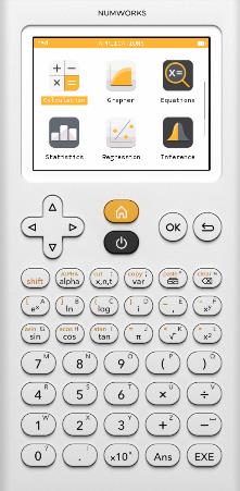
The yellow button above that, with a little picture of a house, takes you to the home menu.

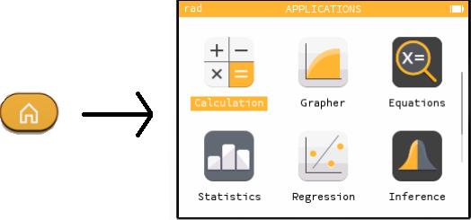
Use the giant impossible-to-miss arrows to move up, down, left, and right.

Then hit either OK or EXE to choose an option. (Side note: I have not yet found any situation where OK and EXE work differently from each other. They seem to be the same button with two different names. Kinda weird.) Anyway, as an example, go to "Calculation" and hit OK if you want to enter equations and have the machine calculate things for you.

A few notes about the home screen.

• You see six options, but there are three more waiting for you if you hit the down-arrow a couple of times.

• Above those six options, way in the upper-left-hand corner—you can see this in my picture above if you look hard—it says rad, indicating that the calculator is in radian mode.
  

  If you go to "Settings" (one of the three menu options hidden below the top six in the home menu), you can change between radian and degree mode.

• The upper-right-hand corner shows your battery charge.

Don't stop reading now. You can't use the calculator until you learn how to enter equations!

Entering Equations

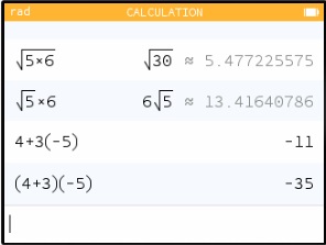
On each line you see the question I typed (at the far left), and the answer the calculator gave (far right). For instance, when I asked for 4+3(-5) the calculator answered -11.

But there are a lot of details hiding in that little screen shot.

• In almost all cases, you type things into the calculator the same way you would write them. If you've used a really ancient calculator (like the TI-30 I had in high school) you might expect to type 5 and then a square root to calculate the square root of 5. Here you start with the square root. This automatically gives you parentheses where you fill in the 5, and you can put other operations around that.

• I didn't actually type 4+3(-5) for the third calculation (although I could have). I typed 4+3×-5. The calculator understands that those are two different notations for describing multiplication, and it displays the one it wants to.

• You can use the "minus" button for two different purposes: to get a negative number (I used it above to get -5), or to subtract two numbers (9-7). That may sound obvious if you've never used a calculator before, but it will come as a surprise if you're used to a TI-83, which uses different buttons for those two purposes.

• The calculator respects the mathematical order of operations. In the third example in the above picture, it multiplied 3×-5 first, and then it added 4, because order of operations says that multiplication comes before addition. In the final example I used parentheses to change that order, so I got a different answer.

• You use the x^y key for exponents, just as you would use the carat (^) on a TI-83.

• The Ans key inserts a variable called ans that means "the last answer I got." So if you type 3+4 and then EXE the calculator displays a 7, but it also loads the number 7 into the variable ans. If the next thing you type is ans+10 you will get the answer 17.

Help! I'm Stuck in a Fraction!

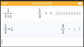
I hope it's clear that the calculator's answers are correct in both cases! But what I want to talk about is how I typed those.

If you type the following keys in the following order:

you get the first calculation I showed above, resulting in the answer 1/3. That's because the ÷ symbol creates a fraction and puts you in the denominator of that fraction. Then, as you keep typing, you're still in the denominator.

And that's great, if that's what you want. If not, the right-arrow key will get you out of the denominator. So the following key sequence produces the second equation above, the one with the answer 3/2.

It's confusing to follow what I'm saying here by just reading. To make it clear, type those two key sequences above on your calculator, and watch what happens at each step. You'll see how that right-arrow changes your cursor location so that the +1 ends up in a different place.

Similar considerations apply to square roots (such as the two different square root equations in the screen shot under Entering Equations above). And the same thing also happens with exponents that you create with the x^y key (consider the difference between 5³⁺¹ and 5³+1). However, the x² key does not move the cursor up into the exponent, so you do not need to follow it with the right arrow.

This is all very different from the TI-83 that I was previously used to. (The TI-83 is much less visual, which causes a whole different set of problems.) But when I switched to the NumWorks, my equations kept coming out wrong. The problem was always this exact issue: I was still typing in the denominator of a fraction, or inside a square root, or up in an exponent, when I didn't mean to be.

At that point, I had to fix the equation that I had incorrectly typed (or was in the middle of incorrectly typing). Which brings me to...

Editing an Equation

If you hit shift and then the backspace key, that clears out your current equation. (Note that the word clear is written on that key in yellow; more on that below.) Hit it again, and that clears out the whole screen.

That may all sound a bit obvious, but here's something that took me more by surprise: you can use the up-arrow to move up into the world of equations you have already entered. Navigate to an old answer or an old equation, and then hit EXE, and that equation will be copied to the bottom of the screen. Then you can mess with it—maybe change a 4 to a 5 or some such, moving around your equation with the arrows and the backspace key—before hitting EXE again to execute it. This is useful if you want to type an equation that is similar to, but not identical to, an equation you already entered.

For even more fun, notice that while you're arrowing around your old equations, many of them have a ... to the right. Click on that to get extra interesting information about that particular result: alternative answers, graphs, prime factorization, whatever the good folks at NumWorks could think of to throw in there.

Shift, Yellow, and Storing Numbers

OK, but what is h anyway? It is a named memory space. Using the ⟶ key (that's shift x^y), you can put a number into memory h.

Here's an example. Suppose that, for some reason, the number 5×(π-2) keeps showing up in your calculations. (Hey, it could happen.) You need to add one to it, you need to double it, all kinds of things...and you don't want to keep typing it! So you type:

5×(π-2)⟶h

This performs the calculation you wanted, and then stores the result in the memory space called h. Thereafter, you can use h in calculations such as:

h+1
2h
1/h+6

...or whatever, you get the idea.

Every letter from a to z can hold its own number. And the capital letters A-Z are different memory spaces, giving you 52 in all.

A few ending notes about this feature.

• If you're in the "Calculation" application and push the var button (top row, more or less just below the on/off button), and then choose "Expressions," you will get a list of all the variables you have defined.

• As you would expect, 2h means the same thing as 2×h. However, if you want to multiply two variables, you must use the times symbol: a×b will give you what you want, but ab will generally give you an error. The NumWorks folks tell me they're going to fix this in a May 2022 update.

• The reason for that strange bug is actually pretty cool: ab might be a different variable! So I lied when I said there was enough space to store 52 numbers: you can store an effectively limitless number of them, with names like money or time. The thing they're going to fix in May is that if you type ab, and you have never defined a variable called ab, then it will look for variables a and b and multiply them.

• Finally, there is a shortcut for the letter x (since it is the variable you will use most often). Instead of hitting alpha and then 2—which will work to get an x but takes two keystrokes—you can get an x with only one keystroke, by hitting the button labeled x,n,t.

Memory Clearing (The Cure-All)

Here's what you do. Go to "Settings" (by going to the home menu and then down-arrowing past the six options you can see to the three options you can't). All the way down at the bottom of the "Settings" menu is an option to "Reset the calculator." That should cure what ails you.

Here's an alternative approach. Look on the back of the calculator. (Make sure it isn't in its case!) In the middle you will see a tiny little hole labeled RESET. Poking into that hole will reset the memory. And here's the point: if you are a teacher who needs to reset 40 of these before a test, you can tell the students to put them on their desks face down, and then walk around and quickly reset them all with an unrolled paperclip.

* * *

At the very top of this page, I advised you to read through the entire "The Basics" section. If you've been reading from the top, congratulations—you have now done that! From here, rather than reading sequentially, I recommend you use the top menu to jump to whatever you need to learn.

Return to the top menu

---

Graphs and Tables

To get you started, let's walk through a simple scenario.

1. From the home menu, choose "Grapher" and you will enter a world with three "tabs" listed at the top: Expressions, Graph, and Table.

2. You want to be in the "Expressions" tab. You may already be there, but if not, up-arrow to the three tabs. (This may take quite a bit of up-arrowing. As a short cut, hit the Back key—it's right next to OK at the top of the calculator—and that will jump you right to the tabs.) Then left-arrow to Expressions and hit EXE.

3. You may now be on "Add an Element." If you aren't, down-arrow until you get to it. Then hit EXE on it, and you get a menu of choices.

4. Choose "Empty" to enter a brand new function.

5. Type a function, using all the usual keys for numbers and operations, and using the x,n,t key for the variable. For instance, the key sequence below will get you the function x²+3. (Note that the x² key does not actually give you x²; it just gives you squared. The x comes from the x,n,t key.)

   

6. Hit EXE to add your function to the list.

7. Up-arrow to "Expressions" (again, the Back key gets you there in one click). Then right-arrow to "Graph" and hit EXE.

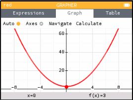
If you're used to an ancient TI-83 like mine, you may suddenly feel like you have moved up in the world: these graphics are vastly better.

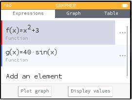
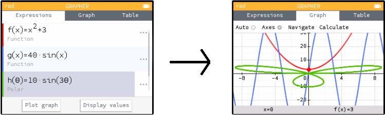
Now, let's say you want to graph more functions. Up-arrow to "Graph" (this may take several up-arrows). Then left-arrow to "Expressions" and hit EXE to go back where you were before, and do it all over again: choose "Add an Element" and add more functions. (You can see in the window below that I have two different functions listed. You can also see, by the way, that they are called f(x) and g(x). I never typed those names; I just typed x²+3 and 40sin(x).)

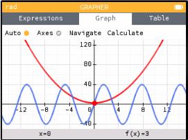
When you "Graph" you will see all of them side by side (just like on a TI-83), in different colors (so much nicer than a TI-83).

Protip: If you look closely at the pictures above, you'll see that in the "Expressions" tab (where I entered the equations), there is a red bar on the left of f(x) and a blue bar on the left of g(x). The calculator is associating each function with a color. You can see those colors in the graphs (in the picture above of the "Graph" tab), and you will see the same colors if you make a table of values.

The Graphing Window

If you want to take tighter control, you can, although I'll admit I find this process a bit painful.

1. While you're looking at your graph, up-arrow to where it says "Auto." (It will reach this before it gets up to "Graph" at the top.) Right-arrow to "Axes" and hit EXE.

2. Arrow down to "Values of X" and hit EXE.

3. You are now on the option "Auto" which is turned on, meaning that the calculator chooses the axes for you. Hit EXE to turn it off. At this point, "Minimum" and "Maximum" below it become available.

4. Arrow down to "Minimum" and hit EXE. Type a new number: the x-value that will define the left side of your screen. Similarly with the maximum x-value.

5. Arrow down to "Confirm" and hit EXE. This pops you up one menu, where you once again arrow down to "Confirm" and hit EXE.

A Table of Values

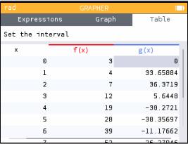
If you look carefully at that picture, you will see that above the table it says "Set the interval." You can arrow to that and hit EXE to set the starting x-value used in the table, and the step size between x-values.

Graphing in Polar Coordinates

1. The first few steps are the same as before. Start in the home menu, choose "Grapher," go to the "Expressions" tab if you're not already there, and choose "Add an element."

2. But now, don't choose "Empty" as before. Instead, down-arrow to the template f(θ)=cos(θ) and hit EXE.

   (As I was following my own directions, I noticed something that could be a bit confusing: I chose a template that said f(θ), but as soon as I hit EXE it became h(θ). That's because the calculator names functions sequentially, and I already had functions named f and g.)

3. In the unlikely event that you want to graph r=cos(θ), just hit EXE a second time. But if you want to graph any other polar function, backspace over the cos(θ) part, leaving the h(θ)= (or whatever yours says) alone. Then type in your new function. The "x,n,t" button will give you a θ in this equation.

4. Once your new function looks right, hit EXE again. Your old functions are still there—for instance, my calculator still has f(x)=x²+3 and g(x)=40 sin(x), since I defined those earlier—but it has now added this polar function. When you go to the "Graph" tab you will see all of them graphed together, each in its own color.

There's one more important feature here, which is that you can specify the domain of your function: that is, the θ-values that will be used in your graph. Here's how you do that.

In the "Expressions" tab, there is a ... to the right of each function. (You can see three of them in my picture above.) Right-arrow onto that ellipsis and hit EXE to get a little menu of options for that particular function. Here you can change the "Plot Restriction," setting the variables θmin and θmax.

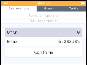
The drawing I showed above has θ going from 0 to 2π. If you (for instance) change θmax to π/2, you will only see part of that polar curve.

Comparison to the TI-83

On the TI-83, you switch into polar "mode." Then all your functions are r(θ) instead of y(x), and the "Window" includes a θ_min and θ_max. On the NumWorks you enter a polar function, but you don't switch into polar mode. This small-sounding difference allows you to do some things on the NumWorks that are not possible on the TI.

• You can display Cartesian and polar graphs together. For instance, you can show that the graph of y=1-x is tangent to the graph r=1-sin θ.

• You can set different θ-domains for each function, rather than treating the θ-domain as a global setting. (By contrast, the minimum and maximum x and y values are global settings, since they define the window you're looking at.)

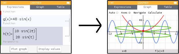
Graphing Parametric Equations

1. The first few steps are the same as before. Start in the home menu, choose "Grapher," go to the "Expressions" tab if you're not already there, and choose "Add an element."

2. But now, don't choose "Empty" as before. Instead, down-arrow to the template and then hit EXE.

   (As I was following my own directions, I noticed something that could be a bit confusing: I chose a template that said f(t), but as soon as I hit EXE it became h(t). That's because the calculator names functions sequentially, and I already had functions named f and g.)

3. In the unlikely event that you want to graph the unit circle, just hit EXE a second time. But if you want to graph any other set of parametric equations, left-arrow your way into the functions. There you will find, possibly to your surprise, that you are in the middle of a 3×2 matrix!
   

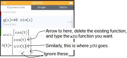
   Edit the two functions that you see, leaving the other four little blank patches blank. The "x,n,t" button will give you a t in this equation.

4. Once your new function looks right, hit EXE again. Your old functions are still there—for instance, my calculator still has f(x)=x²+3 and g(x)=40 sin(x), since I defined those earlier—but it has now added this set of parametric equations. When you go to the "Graph" tab you will see all of them graphed together, each in its own color.

There's one more important feature here, which is that you can specify the domain of your function: that is, the t-values that will be used in your graph. Here's how you do that.

In the "Expressions" tab, there is a ... to the right of each function. (You can see two of them in my picture above.) Right-arrow onto that ellipsis and hit EXE to get a little menu of options for that particular function. Here you can change the "Plot Restriction," setting the variables Tmin and Tmax.

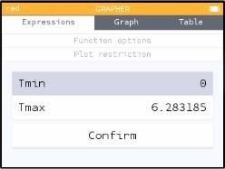
The drawing I showed above has t going from 0 to 2π. If you (for instance) change Tmax to π/2, you will only see part of that parametrically defined curve.

Comparison to the TI-83

On the TI-83, you switch into parametric "mode." Then all your functions are x(t),y(t) pairs instead of y(x), and the "Window" includes a t_min and t_max. On the NumWorks you enter a set of parametric equations, but you don't switch into parametric mode. This small-sounding difference allows you to do some things on the NumWorks that are not possible on the TI.

• You can display Cartesian and parametric graphs together. For instance, you can show that the graph of y=6x-9 is tangent to the graph x = ln t, y = (ln t)².

• You can set different t-domains for each parametric curve, rather than treating the t-domain as a global setting. (By contrast, the minimum and maximum x and y values are global settings, since they define the window you're looking at.)

Curve Fitting, or Regression

1. From the home menu, choose the "Regression" option. This takes you to a screen with three columns (and there are more you can't see to the right), but you're only going to use the first two: the X1 column will have the x-values (or independent variables) of all your points, and the Y1 column the y-values (or dependent variables).

2. Start typing x-values: number, EXE, number, EXE, etc, to fill in the X1 column. Then right-arrow to the Y1 column and do the same.

3. When all your data is entered, up-arrow to where it says "Data," then right-arrow to "Graph" and hit EXE.

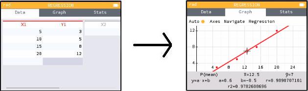
There's another important feature here that is not at all obvious. On the "Data" tab, up-arrow to where it says X1 (above your data but below the tab headings) and hit EXE. This brings you to a menu where you can clear out all the data in the column (which is certainly an important thing to be able to do). But this menu also has a submenu called "Regression" that gives you options besides linear regression. You can find the quadratic curve of best fit, exponential curve, logarithmic curve, and so on.

Return to the top menu

---

Calculus & Advanced Stuff

1. From the home menu, choose the (hopefully-quite-familiar-by-now) "Calculation" option.

2. Now you're going to hit a button that you may not be familiar with. It's called the "Toolbox" and it's on the top row near the right.
   

3. This brings you to a menu with a variety of miscellaneous goodies: absolute value, n^th root, and so on. Down-arrow past those and choose the "Calculus" option, which brings you to yet another menu.

4. Inside that menu, the first option is a derivative. Hit EXE on that, and you are returned to the Calculation screen.

5. Fill in the function you want to take the derivative of, and the x-value at which you want that derivative. Hit EXE again to get your answer.

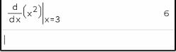
Here's a nifty alternative path. When you're looking at the graph of a function, up-arrow to where it says Auto, and then right-arrow to Calculate. Choose a function, and then toggle on the option "Value of the derivative." When you go back to the Graph, you will see f'(x) displayed at the bottom alongside x and f(x). Similarly, if you hit EXE on the f(x) at the top of a table column, you can switch on a derivative column in the table.

Important note: The calculator uses numerical approximation techniques to find derivatives. In some cases, those techniques will not work, and you will get an answer that is just plain wrong. Caveat emptor.

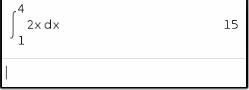
Definite Integrals

1. From the home menu, choose the (hopefully-quite-familiar-by-now) "Calculation" option.

2. Now you're going to hit a button that you may not be familiar with. It's called the "Toolbox" and it's on the top row near the right.
   

3. This brings you to a menu with a variety of miscellaneous goodies: absolute value, n^th root, and so on. Down-arrow past those and choose the "Calculus" option, which brings you to yet another menu.

4. Inside that menu, the second option is an integral. Hit EXE on that, and you are returned to the Calculation screen.

5. Fill in the function you want to integrate, and the limits of integration. Hit EXE again to get your answer.

Important note: The calculator uses numerical approximation techniques to find integrals. In some cases, those techniques will not work, and you will get an answer that is just plain wrong. Caveat emptor.

Imaginary and Complex Numbers

If you are looking for a different answer, choose "Settings" from the home menu. (Can't find it? Go to the home menu and then scroll down, past the six options you see, to find the three other options you don't see.) Inside the Settings menu, go down to "Complex format" and choose "Cartesian."

Now go back and ask for the square root of -1 again, and this time you will get i.

Now that you are in this mode, you can do calculations with i. But look at the screen below. I asked the same-looking question twice—and I was in complex mode both times—but I got different answers. What happened?

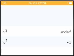
The sneaky answer is that there are two different "i"s (note in the screen shot the slightly different fonts). The first time I hit alpha and then the tan key. That gave me a variable called i, one of the 52 named variables spaces that you can use to store numbers. I hadn't stored anything in that space, so my answer was undefined.

The second time I used the actual i key (second row, next to the log). That is the imaginary number i, not a variable, and its square is -1.

Once you're in complex mode, hit the Toolbox button (pictured below—it's on the top row toward the right) and then go to the "Complex numbers" submenu to find operations such as magnitude and complex conjugate.

Series

1. From the home menu, choose the (hopefully-quite-familiar-by-now) "Calculation" option.

2. Now you're going to hit a button that you may not be familiar with. It's called the "Toolbox" and it's on the top row near the right.
   

3. This brings you to a menu with a variety of miscellaneous goodies: absolute value, n^th root, and so on. Down-arrow past those and choose the "Calculus" option, which brings you to yet another menu.

4. Inside that menu, the third option is the Greek letter Σ (capital sigma) that is used in mathematics to indicate a series. Hit EXE on that, and you are returned to the Calculation screen.

5. Fill in the function that generates terms of your series. The x,n,t button will give you the letter i. Make sure to also fill in the starting and ending i values.

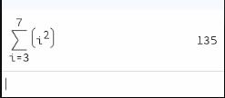
In my example above, the NumWorks has just calculated that 3²+4²+5²+6²+7²=135.

There are also options for working with sequences, including recursively defined sequences.

Matrices

The same memory slots can also hold matrices. Let's store one.

1. From the home menu, choose the (hopefully-quite-familiar-by-now) "Calculation" option.

2. Hit Shift and then the e^x button.
   

   You know by know that hitting Shift before a key activates the function written in yellow on the key. What this key has in yellow is a left square bracket, indicating the opening of a matrix. The calculator gives you a blank 2×2 matrix to fill in.

3. Fill in the numbers (obviously). But what if you don't want a 2×2 matrix? If you fill in a number in the far right column, the calculator will automatically add a new blank column. Similarly with rows, of course. In this way you can extend your matrix to any dimensions you want, always leaving one empty column at the far right and one empty row at the bottom.

4. When your matrix looks the way you want it to, right-arrow out of it. That's when you will see the far-right (empty) column, and the bottom (empty) row, disappear, leaving the matrix you want. But don't hit EXE yet!

5. Hit Shift and then the x^y button to get the right-arrow that means "store," and then hit a letter (using the alpha key).

   Then hit EXE. Now your matrix is stored, associated with that letter.

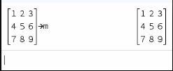
The picture above stores a 3×3 matrix as the variable m.

And now what? You can find matrix operations by hitting the Toolbox button (pictured below—it's on the top row toward the right). That brings you to a menu: choose "Matrices and vectors" and then (under that) "Matrix," and you will find functions to find the inverse and the determinant of your matrix.

More interestingly, you can embed this variable in arbitrarily complicated equations. You will get errors if you do illegal matrix operations (such as taking the inverse of a non-square matrix, adding two matrices with different dimensions, etc). But as long as your matrices fit the operations, the calculator can do wonders. To take a few examples:

• 2a+inverse(b)c will produce one matrix which is a doubled, and another matrix which is the inverse of b multiplied by c, and then add the two. (You can also get that inverse matrix by using x^y and then -1: in other words, type what you would write.)

• det(a)b would take the determinant of a, and multiply it by b, producing and displaying a new matrix; whereas...

• det(a×b) would multiply a times b and then take the determinant of the resulting matrix, producing and displaying a number. (Remember that, as of this writing, you cannot multiply by writing ab: you need that × symbol between them.)

---

Miscellany

Factorial

Solving Equations

1. From the home menu, choose the "Equations" option.

   The resulting screen, and its functionality, should be familiar if you've already done some function graphing. You're looking at a list of equations (although that list may currently be blank).

2. Choose "Add Equation" to add a new equation to the list. From there, you can choose a Template to modify, or you can choose "Empty" and start from scratch.

   When you're typing an equation, you can get an equal sign by hitting shift π. Alternatively, just type a function with no equal sign; when you hit EXE the calculator will supply =0 as the end of your equation.

3. Once you hit EXE on your equation, it is added to the list.

4. Down-arrow to the "Solve the equation" button and hit EXE.

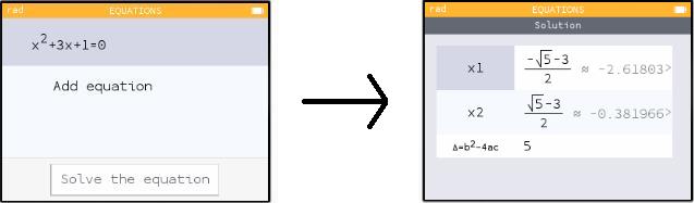
As you can see in my picture above, the calculator solves your equation and gives you one or more answers.

Comparison to the TI-83

The TI-83 offers similar functionality through its "Solver" (well hidden at the bottom of the Math menu). But one thing I always warn students about is that the TI Solver finds only one solution. You give it an x-value, and it hunts near that value until it finds a solution. If you want a different solution, you have to give it a different starting x-value.

By contrast, my picture above shows the NumWorks finding both roots of a quadratic function. I tried a cubic equation and it found all three. Then I tried cos x = x/20. This time the calculator asked me for minimum and maximum x-values. I told it to look between -20 and 20 (which is where all thirteen solutions are). It found ten of them, but warned me that there might be more.

I have no idea what the NumWorks is doing, or what are the limitations of its ability in this area, but it seems to be well out ahead of the TI.

Return to the top menu

---

That's it?

But I have discussed all the functionality that I and my students need—enough to cover you up through BC Calculus. If you have something else you want to know, drop me an email at KenFe@HotMail.com and I'll reply to you and/or add it, if I know the answer!

Send comments or questions to the author