


Next: FFTRN: Multi-Dimensional Real Fourier
Up: How FFTEASY works
Previous: FFTCN: Multi-Dimensional Complex Fourier
The trick to doing a DFT of real data is to once again use the DL
formula. Specifically the routine begins by taking the original array
and passing it as is to fftc1. Of course fftc1 treats the data as an
array of complex numbers. Note, however, that the real parts of those
numbers are the elements of  and the imaginary parts are the
elements of
and the imaginary parts are the
elements of  , so it is possible to extract the actual DFT of
  from the results of fftc1. Let
  represent the output of fftc1
and let
represent the output of fftc1
and let  represent the desired output, i.e. the transform of the
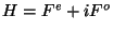
real function . The input we gave to fftc1 was the combination
represent the desired output, i.e. the transform of the
real function . The input we gave to fftc1 was the combination  so by the linearity of Fourier transforms we know that
 . From the DL formula we also know that
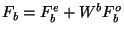 . How can we extract and from
  in order to plug
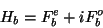
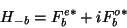
them into the DL formula? The answer lies in the symmetry relation
obeyed by the Fourier transforms of real data (which includes
and ),
in order to plug
them into the DL formula? The answer lies in the symmetry relation
obeyed by the Fourier transforms of real data (which includes
and ),
 . So
. So
 |
(11) |
 |
(12) |
and thus
 |
(13) |
 |
(14) |
Plugging these equations into the DL formula gives
![\begin{displaymath}
F_b = {1 \over 2} \left[H_b + H_{-b}^* - i W^b \left(H_b -
H_{-b}^*\right)\right].
\end{displaymath}](img108.png) |
(15) |
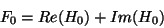
Now all that's left is to figure out where all of these terms are
stored in the array. Remember that all the array indices in these
formulas are complex. In the case of  finding the elements is
trivial because only non-negative values of
finding the elements is
trivial because only non-negative values of  are given as output so
the elements are stored in order
are given as output so
the elements are stored in order
 . (The case
 is treated separately below.) Recall, however, that is
the transform of a complex
is treated separately below.) Recall, however, that is
the transform of a complex  size array, so its elements range
from
size array, so its elements range
from  to
to  in the wrap-around storage order described in
section 2.3.2. In other words the value of
in the wrap-around storage order described in
section 2.3.2. In other words the value of  is stored
in the location
is stored
in the location  . So
. So
![\begin{displaymath}
F_b = {1 \over 2} \left[H_b + H_{N/2-b}^* - i W^b \left(H_b -
H_{N/2-b}^*\right)\right].
\end{displaymath}](img114.png) |
(16) |
Plugging in for  in this equation and noting that
![$W^{N/2-b} = \exp[2 \pi i (N/2-b)/N] = -(W^b)^*$](img115.png) gives
gives
![\begin{displaymath}
F_{N/2-b} = {1 \over 2} \left[H_b^* + H_{N/2-b} - i (W^b)^*
\left(H_b^* - H_{N/2-b}^*\right)\right].
\end{displaymath}](img116.png) |
(17) |
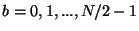
Using these two equations the program steps over all the elements of
the array overwriting and  with and
 . The cases
  and are a little different,
however, because
and are a little different,
however, because  and
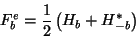
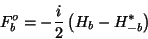
and  are both real. The function fftr1
places in the first (real) slot of the element of the
array and in the second (imaginary) slot. From the formulas
above, noting that
are both real. The function fftr1
places in the first (real) slot of the element of the
array and in the second (imaginary) slot. From the formulas
above, noting that  by periodicity, we see that
 |
(18) |
 |
(19) |
Inverting this process seems like a mess but actually works out to be
nearly identical. I won't reproduce all the algebra here but if you
invert the formulas above to find from you will find that
except for a couple of minus signs and a factor of two for the  and
and  terms the results look identical to the forward case. As a
result the inverse transform simply uses the same loop to rearrange
the array and then calls fftc1 to do an inverse transform and get the
function
terms the results look identical to the forward case. As a
result the inverse transform simply uses the same loop to rearrange
the array and then calls fftc1 to do an inverse transform and get the
function  back.
back.
Next: FFTRN: Multi-Dimensional Real Fourier
Up: How FFTEASY works
Previous: FFTCN: Multi-Dimensional Complex Fourier
Go to The FFTEASY Home
Page
Go to Gary Felder's Home
Page
Send email to Gary at gfelder@email.smith.edu
This
documentation was generated on 2003-09-30