


Next: The Program Potential
Up: Writing Down the Equations
Previous: Writing Down the Equations
The first thing you will need to decide about your model is how to
rescale the variables. In general they are rescaled as
 |
(4.3) |
You may set the variables  ,
,  , and
, and  to whatever you wish. The
variable
to whatever you wish. The
variable  must be set to
  for the program to work correctly,
so this setting is done automatically by the program. If you have in
mind a particular set of rescalings that you think most simplifies
your model then you can simply define these three variables
appropriately. In general, however, there are a set of default values
that should work well for any model where the dominant term is
polynomial in the fields (or can be approximated as such). These
default rescalings are derived and explained in section
6.1.2. Here we simply quote the results. Assuming the
dominant term in your potential is of the form
for the program to work correctly,
so this setting is done automatically by the program. If you have in
mind a particular set of rescalings that you think most simplifies
your model then you can simply define these three variables
appropriately. In general, however, there are a set of default values
that should work well for any model where the dominant term is
polynomial in the fields (or can be approximated as such). These
default rescalings are derived and explained in section
6.1.2. Here we simply quote the results. Assuming the
dominant term in your potential is of the form
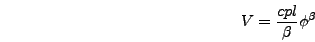 |
(4.4) |
where  is one of the fields in your problem, the default values
for the rescaling variables are
is one of the fields in your problem, the default values
for the rescaling variables are
 |
(4.5) |
where  is the initial value of the field . It is often
most convenient to choose this value such that the derivatives of the
homogeneous fields vanish initially, but this is not necessary.
is the initial value of the field . It is often
most convenient to choose this value such that the derivatives of the
homogeneous fields vanish initially, but this is not necessary.
For the TWOFLDLAMBDA model the dominant term is
 so
so  and
and  . This means that
 |
(4.6) |
From equation (4.5) the time derivative of in
program variables is
 |
(4.7) |
Before running this model on the lattice we solved the ODE for the
evolution of a homogeneous field with
 near the end of inflation and determined that the
expression above equals zero at
near the end of inflation and determined that the
expression above equals zero at
 . (Recall that all
numbers are given here in Planck units.) So we set
. (Recall that all
numbers are given here in Planck units.) So we set  and
for initial conditions set the homogeneous component of
and
for initial conditions set the homogeneous component of  to
zero.
to
zero.
Next: The Program Potential
Up: Writing Down the Equations
Previous: Writing Down the Equations
Go to The
LATTICEEASY Home Page
Go to Gary Felder's Home
Page
Send email to Gary Felder at gfelder@email.smith.edu
Send
email to Igor Tkachev at Igor.Tkachev@cern.ch
This
documentation was generated on 2008-01-21