


Next: Initial Conditions on the
Up: Scale Factor Evolution
Previous: Correcting for Staggered Leapfrog
Power-Law Expansion
LATTICEEASY is designed to self-consistently solve for the evolution
of scalar fields  and the scale factor
  in an expanding
universe. In some cases, however, you may wish to solve for the
behavior of a set of fields in a universe dominated by other forms of
energy, e.g. pure matter or radiation. In this case you can tell the
program to impose a fixed power-law expansion and evolve the fields in
this background. In this section we derive the equations for such an
expansion in program variables. Note that we use the variables
in an expanding
universe. In some cases, however, you may wish to solve for the
behavior of a set of fields in a universe dominated by other forms of
energy, e.g. pure matter or radiation. In this case you can tell the
program to impose a fixed power-law expansion and evolve the fields in
this background. In this section we derive the equations for such an
expansion in program variables. Note that we use the variables  to denote constants of the equations. The in this section have
no relation to the ones in the previous (or any other) section.
to denote constants of the equations. The in this section have
no relation to the ones in the previous (or any other) section.
For a general constant equation of state the scale factor evolution is
given by
 |
(6.37) |
The program time is rescaled as
 |
(6.38) |
which can be inverted to give
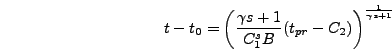 |
(6.39) |
and thus
 |
(6.40) |
To solve for the parameters we want to match the values of
and  at the beginning of the simulation,
  . The scale
factor itself has an arbitrary scaling and is set to
. The scale
factor itself has an arbitrary scaling and is set to  initially,
while the Hubble constant has some well defined initial value
initially,
while the Hubble constant has some well defined initial value
 . The first constraint trivially gives
  . The second
constraint is most easily defined in terms of the program value of the
Hubble constant,
. The second
constraint is most easily defined in terms of the program value of the
Hubble constant,
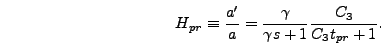 |
(6.41) |
Let  be the value of
  when
when
 |
(6.42) |
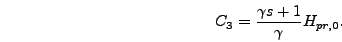
So
 |
(6.43) |
where
 |
(6.44) |
The program value is derived in section 6.3.6
and is automatically calculated by the program. The rescaling variable
 should be defined for your model, so all you need for a power-law
expansion is to specify the value of
should be defined for your model, so all you need for a power-law
expansion is to specify the value of  , which is declared in
parameters.h with the variable name
expansion_power. Note that if you know the equation of
state
, which is declared in
parameters.h with the variable name
expansion_power. Note that if you know the equation of
state  that you want the corresponding power-law
expansion will be given by
that you want the corresponding power-law
expansion will be given by
 |
(6.45) |
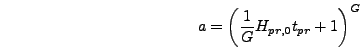
(See for example [4].) If we let
 |
(6.46) |
then the final form of the power-law expansion equations is
 |
(6.47) |
 |
(6.48) |
 |
(6.49) |
The parameters and  are called sfbase and
sfexponent respectively in the program.
are called sfbase and
sfexponent respectively in the program.
Next: Initial Conditions on the
Up: Scale Factor Evolution
Previous: Correcting for Staggered Leapfrog
Go to The
LATTICEEASY Home Page
Go to Gary Felder's Home
Page
Send email to Gary Felder at gfelder@email.smith.edu
Send
email to Igor Tkachev at Igor.Tkachev@cern.ch
This
documentation was generated on 2008-01-21