The function energy() calculates the components of the energy density. The energy density is calculated for all fields regardless of the value of noutput_flds. The output is in two files, one for the components of energy density and one for monitoring energy conservation.
The components are output to a file called energy_ext. The
number of columns in this file varies with the number of fields and
with the number of terms in the potential. Specifically, the first
column contains the time, the next nflds columns contain
the kinetic energy
 , the next nflds columns contain the
gradient energy
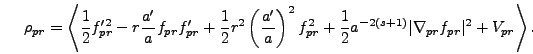
, the next nflds columns contain the
gradient energy
![]() , and the
remaining columns contain the potential terms. The kinetic and
gradient energies are calculated by energy(), whereas the
potential energy is calculated by a model-specific function called
potential_energy() in model.h. The output is in
program units, meaning
, and the
remaining columns contain the potential terms. The kinetic and
gradient energies are calculated by energy(), whereas the
potential energy is calculated by a model-specific function called
potential_energy() in model.h. The output is in
program units, meaning
| (5.42) |
 |
(5.43) |
The second file generated by energy() is called
conservation_ext. The first column contains the time and
the second column contains a quantity used to monitor energy
conservation. For the case of no expansion (Minkowski space) this
quantity is simply the ratio of total energy density to energy density
at the beginning of the run. Of course this quantity should remain
close to ![]() throughout the run. In an expanding universe the
situation is a little more complicated because energy density is not
conserved, but rather decreases in a way determined by the expansion
rate and the equation of state of the fields. This redshifting of
energy is described by the continuity equation
throughout the run. In an expanding universe the
situation is a little more complicated because energy density is not
conserved, but rather decreases in a way determined by the expansion
rate and the equation of state of the fields. This redshifting of
energy is described by the continuity equation
| (5.45) |
| (5.46) |
In the case of fixed power-law expansion the conservation file is not created.